Mipmap selection in too much detail
In this post, I want to shed some light on something I’ve been wondering about for a while: How exactly are mipmap levels selected when sampling textures on the GPU? If you already know what mipmapping is, why we use it, and what pixel derivatives (ddx() / ddy()) are, you can skip to the section Derivatives to mipmap levels. The post does, however, assume some knowledge of graphics programming.
Mipmapping primer
A very common operation in shaders is texture sampling. In HLSL, we typically use the Texture2D.Sample() function for this. For a regular 4-channel floating-point texture, the full function signature looks like this:
float4 Texture2D.Sample(SamplerState sampler, float2 location);
It takes as input a location to sample the texture at, and a SamplerState, which is an object containing metadata used to influence the sampling, like which texture filtering mode should be used.
Here is an example of a simple fragment shader which shades each pixel by sampling a texture _Texture using the texture coordinates in the 0th UV channel:
float4 frag (float2 uv : TEXCOORD0) : SV_Target
{
    return _Texture.Sample(sampler_Texture, uv);
}
When applied to a quadrilateral and fed a brick texture as input, we get this:
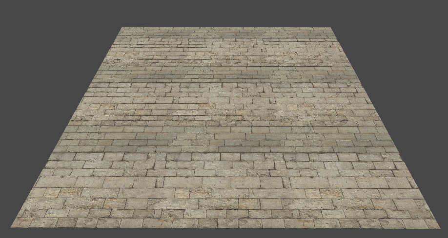
Notice that the surface looks rather ‘pixelated’, especially near the far edge. This is called texture aliasing. The root cause is that the size of the texture space region covered by a screen pixel varies with distance and viewing angle.
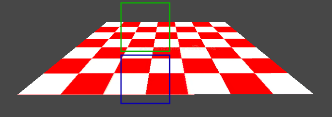
Consider, for illustration, the tilted quadrilateral. Observe how the same area in screen space can correspond to very different areas in texture space. The blue square covers roughly 4 pixels, while the green one covers roughly 12, even though they have the same area in screen space.
The more shallow the viewing angle, the more texels are covered by each pixel on the screen. Since we only sample 1 texel for every screen pixel, most of the texels covered by the screen pixel are aliased into a single sample - the contribution from the covered texels that were not sampled is lost!
The typical solution to this is mipmapping - we first generate a bunch of smaller versions of our texture, called mipmaps, by averaging texels from the higher resolution texture. As the mipmaps get smaller, their contents get more blurry. We are effectively applying a series of low-pass filters to the texture. We typically name the mipmaps using numbers, where 0 is the full resolution texture, and each subsequent number corresponds to a lower resolution texture. I’ll call these numbers ‘mipmap levels’.
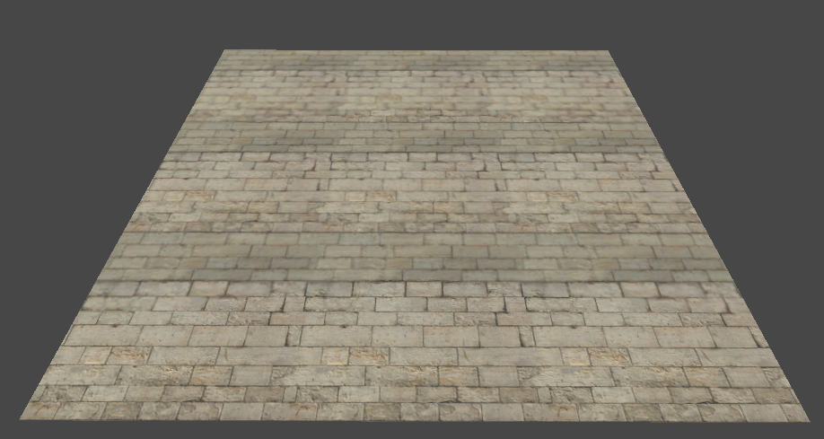
 In cases where texture sampling would result in aliasing, because too many texels are covered by the screen pixel, we instead sample a lower resolution mipmap to mitigate it. That way, we get an approximate average of the texels in the covered area. Here’s the same setup as before, but now with mipmapping enabled:
 I didn’t have to change the shader at all to achieve this - when
 Texture2D.Sample() is used, and the input texture contains mipmaps, the GPU will automatically select an appropriate mipmap level for each sample!
If you are like me, you won’t find this explanation very satisfying. The GPU does some magic to select a mipmap level? Ok - so how does it work? That’s what the rest of this post is about.
Pixel derivatives
A common mental model for a fragment shader is “the piece of code inside of a big parallel for-loop iterating over every pixel on the screen”. The fragment shader is invoked for every pixel in parallel; each invocation gets a set of per-pixel inputs, and uses them to calculate the final color at that pixel. This is a fine mental model, but it doesn’t tell the full story.
In reality, fragment shaders aren’t invoked for every pixel in isolation - rather, they are invoked for 2x2 blocks of pixels, typically called “pixel quads”, or just “quads”. This setup allows us to approximate partial derivatives in screen space for any variable using the finite difference method! In HLSL, the functions to do this are called ddx() and ddy(), and return partial derivatives along the X and Y axes in screen space, respectively. You couldn’t implement these functions yourself - they are magic intrinsics which are implemented in hardware by subtracting the values associated with different pixels in the quad.
Now, observe what happens if we apply a small fragment shader that visualizes the partial derivatives along the Y-axis of the UV coordinates we were using to sample the texture from earlier:
float4 frag (float2 uv : TEXCOORD0) : SV_Target
{
    // Multiply by 15 so we can actually see the derivatives,
    // they are typically very small.
    return float4(ddy(uv), 0, 1) * 15;
}
The more shallow the viewing angle, the larger the partial derivatives get. Additionally, the partial derivatives are larger further away from the camera. ![]()
These conditions line up well with the cases where texture sampling would result in ugly aliasing, so it shouldn’t come as a big surprise that the selection of mipmap levels has something to do with the partial derivatives of the input coordinates used to sample the texture. In fact, Texture2D.Sample() can be seen as syntax sugar for the more general Texture2D.SampleGrad() function:
// These 2 lines of code are equivalent:
Texture2D.Sample(sampler, location);
Texture2D.SampleGrad(sampler, location, ddx(location), ddy(location));
Texture2D.SampleGrad() takes the partial derivatives of the sampling location explicitly, whereas Texture2D.Sample() implicitly calculates them using ddx() and ddy(). Passing these explicitly can be useful in cases where the sampling locations are warped in a way that prevents ddx() and ddy() from returning useful partial derivatives (for example, during textured raymarching or parallax mapping). It also lets us use analytical partial derivatives in cases where we have a way to compute them.
This description still leaves an open question: How exactly does Texture2D.SampleGrad() use the input partial derivatives to determine which mipmap level to sample?
Derivatives to mipmap levels
Texture2D.SampleGrad() has some internal logic that maps from the partial derivatives of the sampling location to a specific mipmap level. This function directly corresponds to a hardware instruction on the GPU, though, so we unfortunately can’t just ‘look at the code’. To get a better idea of how it works, we can ask 2 questions: What does the mapping look like conceptually, and what does the hardware do in practice? Both questions are surprisingly difficult to find good answers to online, but I’ll tackle them both one by one.
What does the mapping look like conceptually?
One place you might think to look for information on how the mapping should work, is in the spec for your graphics library of choice. I find the GLES3.0 spec particularly readable. According to section 3.8.10.1 “Scale Factor and Level of Detail”, the mipmap level is calculated like so:
\[MipLevel(x, y) = log_2(\rho(x, y))\]Where \(x, y\) are the coordinates of the screen pixel, and \(\rho\) is a “scale factor” defined by:
\[\rho = max\Bigg\{\sqrt{\bigg(\frac{\partial u}{\partial x}\bigg)^2 + \bigg(\frac{\partial v}{\partial x}\bigg)^2},\sqrt{\bigg(\frac{\partial u}{\partial y}\bigg)^2 + \bigg(\frac{\partial v}{\partial y}\bigg)^2}\Bigg\}\]Here, \(u\) and \(v\) denote the coordinates of the sampling location in texture space, scaled to the range \([0; TextureSize]\), so \(\frac{\partial u}{\partial x}\) for example is the partial derivative of the horizontal coordinate of the sampling location with respect to the \(x\), i.e. ddx(u * textureSize).
That’s a bit of a mouthful, so let’s translate it to code:
float MipLevel(float u, float v, float textureWidth, float textureHeight)
{
    float du_dx = ddx(u * textureWidth);
    float dv_dx = ddx(v * textureHeight);
    float du_dy = ddy(u * textureWidth);
    float dv_dy = ddy(v * textureHeight);

    float lengthX = sqrt(du_dx*du_dx + dv_dx*dv_dx);
    float lengthY = sqrt(du_dy*du_dy + dv_dy*dv_dy);
    float rho = max(lengthX, lengthY);

    return log2(rho);
}
This should be somewhat intuitive - as the magnitude of the partial derivatives increase, so should the mipmap level. We only really care about the axis where the aliasing will be worst (the axis with the largest magnitude), hence the max(). The log2() accounts for the fact that each increment in mipmap level corresponds to sampling a texture that is half the size.
If you search around the web for how to calculate mipmap level manually, you will probably find a solution like this. However, as we will soon see, this is not the full story.
What does the hardware actually do?
Since Texture2D.SampleGrad() is implemented in hardware, we can’t look at the implementation directly. However, we can use observations of its behavior to deduce what it is doing. To facilitate this, I will first need a texture with mipmaps that are easily distinguishable from each other. Luckily, most graphics frameworks let you manually fill in the texture data for each mipmap - they don’t have to be blurry versions of the full-resolution texture. Since I’m using Unity for visualization, I wrote a little script that produces a texture where each mipmap is a single, bright, clearly distinguishable color. The resulting texture looks like this:
Next, I wrote a shader that samples the texture using Texture2D.SampleGrad(), but where the sampling location is a constant, and the partial derivatives are based on UV coordinates. Texture2D.SampleGrad() takes a partial derivative of the sampling location for both the X and Y axes, each of which are 2-dimensional vectors, so this is technically a 6-dimensional function. Since we are keeping the sampling location fixed, it is a 4-dimensional function in practice. Functions of over 3 dimensions are a bit tricky to visualize, so I’ll focus on just the partial derivatives for the X axis for now, and leave the Y axis partial derivatives as 0:
float4 frag (float2 uv : TEXCOORD0) : SV_Target
{
    // Scale UVs from [0; 1] to [-1; 1]
    float2 scaledUV = (uv - 0.5) * 2.0;

    // Sample texture at location (0.5, 0.5),
    // using X derivative = UV coords,
    // and Y derivative = 0.
    float2 samplingLocation = 0.5;
    float2 yDerivative = 0;
    float4 hardwareSample = _MainTex.SampleGrad(
        sampler_MainTex,
        samplingLocation,
        scaledUV.xy,
        yDerivative);

    return hardwareSample;
}
Applying this shader to a quadrilateral gives this result on my machine (GPU is an RTX 4070 super):
 The image is scaled such that the bottom left corner corresponds to X-axis partial derivatives of (-1, -1), and the top right corner corresponds to (1, 1). The color at each pixel indicates which mipmap level is being sampled, when
 Texture2D.SampleGrad() is passed partial derivatives equal to the pixel coordinates.
When I first saw this result, I was a bit surprised. Why are there jagged edges!? The formulas described in the previous section should result in a bunch of perfect concentric circles! As it turns out, current graphics libraries leave the specifics of the implementation up to the GPU vendor, and only prescribe some loose criteria on the implementation. Nvidia cards use a particularly crude approximation.
Side note: This is just one of many pieces of functionality that differ in implementation across different vendors. It’s a pet peeve of mine when people assume that there is a “one true correct” implementation of pretty much anything in GPU-land. To name a few other areas where vendors differ: The precision of transcendentals like
cos(x)andsin(x), the implementation of AlphaToCoverage (AMD uses dithering), subtle differences in rasterizer output, especially with conservative rasterization, etc. This is unfortunately a big source of pain when doing image-based/golden-image testing for anything involving the graphics pipeline, and is one of the big reasons such test setups often have per-platform reference images, and use fuzzy comparisons.
My next instinct was to determine which vendors actually differ in their implementation, and to what extent. I asked a bunch of friends to try it on their hardware and collected the results. I’m only rendering the quadrant with positive partial derivatives here, since the shape is symmetric anyway:
A few notes on my findings:
- All tested vendors seem to roughly agree on the mapping function. Every image resembles a set of concentric circles with the same radius. The extent to which the circle is approximated differs quite a bit across every vendor, though.
- No two vendors agree entirely on the implementation.
- All tested vendors seem to be consistent across their hardware lineup. Interestingly, AMD’s APUs are consistent with their dedicated GPUs.
- The result is the same across all the graphics libraries Unity supports (I checked).
And with this, I present perhaps the first-ever GPU tier list ranked in order of fidelity of partial-derivative-to-mipmap-level-mapping-function (the only important metric, clearly): Adreno/Qualcomm > AMD > Intel > MacBook/Apple > Nvidia. You heard it here first, Nvidia hardware bad! (/s)
Exploring the full 4D mapping function
In the previous visualizations of the partial-derivative-to-mipmap-level mapping function, I’ve only visualized the influence of X-axis partial derivatives and have left the Y-axis partial derivatives at (0, 0). Next, I’d like to visualize the influence of both axes simultaneously. The easiest way I found to visualize this 4-dimensional function is using a grid. In each grid cell, we will have an image where the X-axis partial derivatives vary. Each grid cell will use fixed values for the Y-axis partial derivative, the values depending on the location of the cell. This way, we can see 2-dimensional “slices” of the full function. I whipped up a Unity script to render that out using the shader from earlier, which produced this image:
Note: This kind of visualization will pop up several times throughout the post, so it’s worth hammering in what we are looking at: The bottom left grid cell has constant Y-axis partial derivatives (0, 0), while the top right grid cell has constant Y-axis partial derivatives (1,1), all the cells between have constant Y-axis partial derivatives somewhere between 0 and 1. Within each grid cell, the local X and Y coordinates determine the X-axis partial derivatives. I’m only visualizing positive Y-axis partial derivatives, because the images for negative partial derivatives are just the same, but mirrored. The color once again indicates the selected mipmap level. Of course, this image is very vendor-specific - these images were all generated on an RTX 4070 Super.
With this setup, we can easily compare what the hardware does to the proposed software implementation from the What does the mapping look like conceptually? section, using Texture2D.SampleLevel() to explicitly sample the mipmap level we have selected. Here’s the same image, but using the software implementation:
 That looks… quite different from the hardware implementation. As expected, the software implementation produces perfect circle patterns, while the hardware implementation approximates them. But additionally, the hardware implementation produces some kind of ellipse shape whenever both the X- and Y-axis partial derivatives have nonzero components, while the software implementation only ever produces perfect circles. This surprised me a bit when I first saw it, since I found no mention of this behavior during my initial research. This piqued my interest and drove me to attempt to reverse engineer the behavior. The answers were out there, I just had to dig a little deeper…
Reverse engineering the hardware implementation
The first resource I managed to find, which made mention of an ellipse in the context of mipmap level selection, was the DirectX 11.3 Functional Spec (praise be), in Section 7.18.11 “LOD Calculations”. I’ll briefly restate the relevant parts of the spec, then dissect them:
- Given a pair of partial derivative vectors representing an elliptical transform, it is important to calculate LOD using a proper orthogonal Jacobian matrix, as described by Heckbert 89. When performing anisotropic filtering, it is also important to use these modified vectors to calculate the proper filtering footprint. D3D11.3 will allow approximations to this effect. The following describes the ideal transformation, given 2-dimensional vectors:
Implicit ellipse coefficients:

A = dX.v ^ 2 + dY.v ^ 2
B = -2 * (dX.u * dX.v + dY.u * dY.v)
C = dX.u ^ 2 + dY.u ^ 2
F = (dX.u * dY.v - dY.u * dX.v) ^ 2
- Defining the following variables:
p = A - C
q = A + C
t = sqrt(p ^ 2 + B ^ 2)
- The new vectors may be then calculated as:
new_dX.u = sqrt(F * (t+p) / ( t * (q+t)))
new_dX.v = sqrt(F * (t-p) / ( t * (q+t)))*sgn(B)
new_dY.u = sqrt(F * (t-p) / ( t * (q-t)))*-sgn(B)
new_dY.v = sqrt(F * (t+p) / ( t * (q-t)))
- The following caveats also apply:
- if either of dX or dY are of zero length, an implementation should skip these transformations.
- if dX and dY are parallel, an implementation should skip these transformations.
- if dX and dY are perpendicular, an implementation should skip these transformations.
- if any component of dX or dY is inf or NaN, an implementation should skip these transformations.
- if components of dX and dY are large or small enough to cause NaNs in these calculations, an implementation should skip these transformations.
- if(ComputeIsotropicLOD), the LOD calculation is:
float lengthX = sqrt(dX.u*dX.u + dX.v*dX.v + dX.w*dX.w)
float lengthY = sqrt(dY.u*dY.u + dY.v*dY.v + dY.w*dY.w)
output.LOD = log2(max(lengthX,lengthY))
Phew, that’s a bit of a mouthful… In the snippets from the spec, dX and dY represent the X- and Y-axis partial derivatives we’ve discussed previously. The w component of these vectors is only used for 3D- and cubemap textures, so it isn’t relevant here. Notice that the code in the very last snippet looks almost exactly like the software implementation we tested earlier. However, most of the text before that snippet describes some kind of ‘elliptical’ transformation that should be applied to the partial derivatives before we calculate their lengths. This sounds quite promising, so let’s try to grok what the spec is prescribing.
Missing elliptical transformation
Side quest: Texture filtering theory and vector calculus
Before I can describe the elliptical transformation, we need to visit a few ideas from the theory of texture filtering and from vector calculus. If you are already familiar with jacobians and the concept of pixel footprint, you can probably skip to the next section Understanding the elliptical transformation.
A naïve approach to rendering a textured surface is this: For each screen pixel, determine the corresponding point on the surface, find its corresponding point in texture space, then read the value in the texture nearest to this point. As we’ve established earlier, this approach causes aliasing; when a screen pixel covers too many texels, and only one texel is sampled, the contribution from most of the covered texels is lost. A better approach would be to integrate over the area covered by each screen pixel, gathering contribution from all the covered texels. Mipmapping is a cheap way to approximate this integral using precomputed tables.
Ideally, we’d like to integrate over the projection of the screen pixel onto the texture. This projection is called the “footprint” of the pixel. To do this, we want to know how a unit area in screen space (i.e., a pixel) is transformed when projecting into texture space. The typical mathematical tool for describing changes in area due to mappings between spaces, such as projection, is called “the jacobian matrix” or just “the jacobian”. When used to transform a point, the jacobian of the mapping provides the best linear approximation of the mapping at that point. When the jacobian is a square matrix, its determinant describes how much space is ‘stretched’ at that point. The jacobian is constructed from first-order partial derivatives of coordinates in the input space with respect to coordinates in the output space. In our case, the input space is screen space, and the output space is texture space. The jacobian looks like this:
\[\Large \begin{bmatrix} \frac{\partial u}{\partial x} & \frac{\partial u}{\partial y} \\ \frac{\partial v}{\partial x} & \frac{\partial v}{\partial y} \end{bmatrix}\]Where \((u, v)\) are coordinates in texture space, and \((x, y)\) are coordinates in screen space. If you’ve paid attention so far, this might ring a few bells - these partial derivatives can be calculated in HLSL using ddx() and ddy(). In other words, we can view the partial derivatives passed to Texture2D.SampleGrad() as forming a jacobian which describes the projective mapping involved in rendering the textured surface.
In reality, it is impractical to integrate over the actual footprint of a screen pixel, as it will in general be a curvilinear quadrilateral (a quadrilateral with curved edges) - quite an unpleasant shape. Therefore, most approaches approximate it as either a regular quadrilateral or an ellipse, as illustrated in the figure below (Image source).
 When using mipmapping, we are mostly interested in the size of the footprint. The larger the area, the larger mipmap level we need to use, since higher mipmap levels correspond to approximations of integrals over larger regions of the texture.
Understanding the elliptical transformation
With these concepts in mind, let us dissect the elliptical transformation described in the DirectX 11 spec. The first paragraph reads:
“Given a pair of partial derivative vectors representing an elliptical transform, it is important to calculate LOD using a proper orthogonal Jacobian matrix, as described by Heckbert 89.”
I’ve highlighted the 2 important concepts with bold text. We have the partial derivatives of our texture sampling coordinates, but in what sense do these represent an elliptical transform? Imagine representing each screen pixel with a unit circle described by an angle \(\theta\), such that \(s(\theta)\) evaluates to all the points on the perimeter of the unit circle:
\[\Large s(\theta)= \begin{bmatrix} cos(\theta) \\ sin(\theta) \end{bmatrix}\]If we additionally construct the jacobian described in the previous section:
\[\Large \begin{bmatrix} \frac{\partial u}{\partial x} & \frac{\partial u}{\partial y} \\ \frac{\partial v}{\partial x} & \frac{\partial v}{\partial y} \end{bmatrix}\]… And transform the unit circle with the jacobian via matrix multiplication to get a new function:
\[\Large p(\theta) = \begin{bmatrix} \frac{\partial u}{\partial x} & \frac{\partial u}{\partial y} \\ \frac{\partial v}{\partial x} & \frac{\partial v}{\partial y} \end{bmatrix} \begin{bmatrix} cos(\theta) \\ sin(\theta) \end{bmatrix}\]The resulting function \(p(\theta)\) will describe an ellipse, where the 2 column vectors of the jacobian (i.e., the X- and Y-axis partial derivatives) are on the perimeter of the ellipse. In the special case where the column vectors are perpendicular and have the same length, the result is still just a (potentially scaled) circle. When the column vectors are perpendicular, but have different lengths, the result is an ellipse where the column vectors are the semi-major and semi-minor axes of the ellipse. If the vectors are not perpendicular, this doesn’t apply.
That explains the first part of the paragraph, so what is the “proper orthogonal Jacobian matrix” part about? When the column vectors of the jacobian are not perpendicular, the jacobian does not form an orthogonal basis - shapes transformed by the jacobian will be sheared. Recall that selecting a mipmap level involves calculating 2 lengths - in our software implementation from earlier, this was done like so:
float lengthX = sqrt(du_dx*du_dx + dv_dx*dv_dx);
float lengthY = sqrt(du_dy*du_dy + dv_dy*dv_dy);
When the column vectors of the jacobian are perpendicular, this code calculates the distance to the furthest point on the perimeter of an ellipse, whose semi-major and semi-minor axes are given by the column vectors. You can think of this as measuring how ‘stretched’ the ellipse is, along whichever axis is most stretched. That’s exactly what we want for mipmapping - the more stretched the elliptical footprint, the more texels it will cover, and the higher the mipmap level we need. However, when the column vectors are not perpendicular, the shearing breaks this stretch metric. We need to manually correct for this by calculating the metric in a different coordinate system. To do this, we need to diagonalize the ellipse.
Diagonalizing an ellipse means finding a coordinate system in which the ellipse is aligned with the axes. In particular, the major and minor axes should be aligned with the X and Y axis of the coordinate system. This eliminates the shearing, and allows us to calculate the stretch metric properly.
Note: For the curious reader, this ‘diagonalization’ is closely related to matrix diagonalization, which decomposes a matrix into its eigenvectors and eigenvalues. In fact, ellipses can be represented as a 2x2 matrix whose eigenvectors give the direction of the major and minor semi-axes, and whose eigenvalues are related to the length of the axes.
The next few paragraphs of the DirectX 11 spec describe an algorithm for performing this diagonalization, taken from Heckbert 89. The details of this algorithm are not so important, so I won’t describe them. Instead, to build intuition, I have implemented the algorithm in a graphing calculator, which lets us easily see what is going on:
Note: You can play with this interactive demo here.
The image shows an elliptical footprint corresponding to a case where the X- and Y-axis partial derivatives (labelled \(d_x\), \(d_y\)) are not perpendicular. Notice how their length no longer describes the stretch of the ellipse. The outputs of the algorithm (labelled \(n_x\), \(n_y\)) are a set of new basis vectors describing the transformation to a coordinate space in which the ellipse is axis-aligned. These new basis vectors are the column vectors of our “proper orthogonal Jacobian matrix”. This new jacobian describes almost the same mapping as the original one, and would produce the exact same ellipse as the original when used to transform the unit circle. The only difference is where the basis vectors are pointing.
This visualization also shows why the DirectX spec provides a bunch of corner cases where the diagonalization should not be applied:
The following caveats also apply:
- if either of dX or dY are of zero length, an implementation should skip these transformations.
- if dX and dY are parallel, an implementation should skip these transformations.
- if dX and dY are perpendicular, an implementation should skip these transformations.
- if any component of dX or dY is inf or NaN, an implementation should skip these transformations.
- if components of dX and dY are large or small enough to cause NaNs in these calculations, an implementation should skip these transformations.
If either partial derivative is zero length, the coordinate would be flattened to an infinite line.
 The same happens if the partial derivatives are parallel:
 If the partial derivatives are perpendicular, there is no shearing, so performing the diagonalization is a waste of effort. Other than that, the final 2 points about inf and NaN are pretty self-explanatory.
With the elliptical transformation under our belt, let’s try adding it to our software implementation of mipmap level selection from earlier:
void EllipseTransformDerivatives(inout float2 dx, inout float2 dy)
{
    bool anyZero = length(dx) == 0 || length(dy) == 0;
    bool parallel = (dx.x * dy.y - dx.y * dy.x) == 0;
    bool perpendicular = dot(dx, dy) == 0;
    bool nonFinite = isinf(dx) || isinf(dy) || isnan(dx) || isnan(dy);
    if (!anyZero && !parallel && !perpendicular && !nonFinite)
    {
        float A = dx.y*dx.y + dy.y*dy.y;
        float B = -2.0 * (dx.x * dx.y + dy.x * dy.y);
        float C = dx.x*dx.x + dy.x*dy.x;
        float F = (dx.x * dy.y - dy.x * dx.y) * (dx.x * dy.y - dy.x * dx.y);
        float p = A - C;
        float q = A + C;
        float t = sqrt(p*p + B*B);
        float2 newDx, newDy;
        newDx.x = sqrt(F * (t+p) / ( t * (q+t)));
        newDx.y = sqrt(F * (t-p) / ( t * (q+t)))*sign(B);
        newDy.x = sqrt(F * (t-p) / ( t * (q-t)))*-sign(B);
        newDy.y = sqrt(F * (t+p) / ( t * (q-t)));

        bool failed = any(isnan(newDx) || isinf(newDx) || isnan(newDy) || isinf(newDy));
        if (!failed)
        {
            dx = newDx;
            dy = newDy;
        }
    }
}
Rendering out the same visualization we used before:
 This looks a lot more similar to what the hardware implementation was doing!
Trilinear filtering
All the visualizations I’ve made thus far have been without any kind of hardware texture filtering, and just use simple nearest-neighbor interpolation. Enabling bilinear filtering makes no difference, as it doesn’t affect how the mipmap level is selected. Enabling trilinear filtering, however, does make a difference. Rendered with the correct software implementation:
 And with hardware mipmap level selection:
 Trilinear filtering is just like bilinear filtering, but where we additionally interpolate between 2 mipmap levels. Without trilinear filtering, the selected mipmap level is just rounded to the nearest integer, and only one mipmap is sampled. With trilinear filtering, the floor and ceiling of the mipmap level are calculated, the 2 corresponding mipmaps are sampled, and the results are linearly interpolated using the fractional part of the mipmap level. This is why we’ve been calculating it as a
 float all along.
With that, harsh transitions between mipmap levels from the previous images are changed to smooth gradients. This is not very surprising, but I wanted to show that the software implementation continues to hold up when using trilinear filtering.
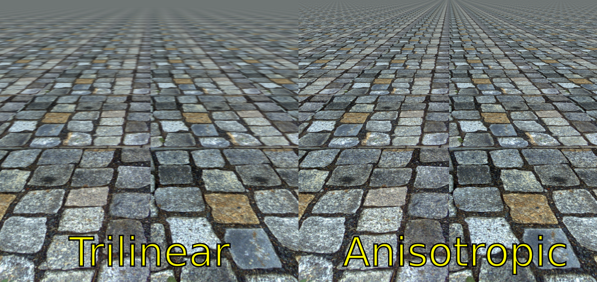
Anisotropic filtering
In addition to bilinear and trilinear filtering, most GPUs also support anisotropic filtering. Anisotropic filtering aims to alleviate one of the main issues with mipmapping. Mipmapping reduces aliasing from texture samples, but also introduces blurring, especially at shallow viewing angles. Anisotropic filtering effectively removes the blur by taking multiple texture samples from a higher resolution mipmap when the footprint of a pixel is unevenly stretched (Image source):
 The typical algorithm for anisotropic filtering works like this:
- Determine the elliptical footprint of the screen pixel using the X- and Y-axis partial derivatives of the sampling location in texture space.
- Determine the semi-major and semi-minor axes of the ellipse. The semi-major (longer) axis is called the “axis of anisotropy”.
- Calculate the ratio of the lengths of the semi-major and semi-minor axes. This is called the “ratio of anisotropy”.
- Clamp the ratio of anisotropy to the maximum degree of anisotropy - this is typically a setting on the texture, with possible values ranging from 0 to 16. The maximum degree is sometimes called the “aniso level”.
- Calculate \(log_2(semiMinorAxisLength)\). This is the mipmap level to sample.
- Distribute sample points along the axis of anisotropy. The number of sample points depends on the clamped ratio of anisotropy.
- Sample the texture at each of the sample points and average their values.
Notice that, unlike with regular mipmapping, where we use the length of the semi-major axis to select the mipmap level, we now use the length of the semi-minor axis. This is what mitigates the blurring caused by mipmapping - we sample a higher resolution texture when the pixel’s footprint is anisotropic (stretched differently on each axis). That alone would just reintroduce aliasing, so to mitigate this, we take more samples along the axis where they are needed most, effectively mitigating the added aliasing by supersampling, rather than blurring.
So, how does enabling anisotropic filtering change the visualization of mipmap level selection from before? To visualize this, I’ve upgraded our previous visualization to an animation. Since anisotropic filtering is parameterized by a maximum degree of anisotropy setting, the visualization is now an animation. Each maximum degree produces a different image:
 When the maximum degree of anisotropy exceeds 0, the image no longer matches what our software implementation produced. This makes sense - anisotropic filtering affects mipmap level selection, but our implementation isn’t accounting for it.
Returning to the DirectX 11 spec, recall that the paragraph about the elliptical transform read: “[…] it is important to calculate LOD using a proper orthogonal Jacobian matrix, as described by [Heckbert 89]. When performing anisotropic filtering, it is also important to use these modified vectors to calculate the proper filtering footprint.”. I skipped over this part earlier, but it is exactly what we are missing. The spec further elaborates: “if(ComputeAnisotropicLOD), the LOD calculation is:”
// Compute outputs:
// (1) float ratioOfAnisotropy
// (2) float anisoLineDirection
// (3) float LOD

float squaredLengthX = dX.u*dX.u + dX.v*dX.v
float squaredLengthY = dY.u*dY.u + dY.v*dY.v
float determinant = abs(dX.u*dY.v - dX.v*dY.u)
bool isMajorX = squaredLengthX > squaredLengthY
float squaredLengthMajor = isMajorX ? squaredLengthX : squaredLengthY
float lengthMajor = sqrt(squaredLengthMajor)
float normMajor = 1.f/lengthMajor

output.anisoLineDirection.u = (isMajorX ? dX.u : dY.u) * normMajor
output.anisoLineDirection.v = (isMajorX ? dX.v : dY.v) * normMajor

output.ratioOfAnisotropy = squaredLengthMajor/determinant

// clamp ratio and compute LOD
float lengthMinor
// maxAniso comes from a Sampler state.
if (output.ratioOfAnisotropy > input.maxAniso)
{
    // ratio is clamped - LOD is based on ratio (preserves area)
    output.ratioOfAnisotropy = input.maxAniso
    lengthMinor = lengthMajor/output.ratioOfAnisotropy
}
else
{
    // ratio not clamped - LOD is based on area
    lengthMinor = determinant/lengthMajor
}

// clamp to top LOD
if (lengthMinor < 1.0)
{
    output.ratioOfAnisotropy = MAX(1.0, output.ratioOfAnisotropy*lengthMinor)
}

output.LOD = log2(lengthMinor);
I’ve omitted some comments for brevity. The spec states that this code should run after applying the elliptical transformation from earlier. This is a pseudocode implementation of (part of) the algorithm for anisotropic filtering described earlier. It produces the ratio of anisotropy (ratioOfAnisotropy), the axis of anisotropy (anisoLineDirection), and the mipmap level (LOD).
To illustrate this, I’ve extended my interactive ellipse diagram from earlier with an implementation of the algorithm. As the partial derivative vectors move around, the axis of anisotropy remains the major axis of the ellipse, and the selected mipmap level depends on the size of the minor axis.
Note: You can play with the updated version of the diagram here.
For now, only the portions of the pseudocode from the DirectX spec relating to mipmap level calculation are relevant. This pseudocode is straightforward to translate into real shader code. Doing so yields the following:
 Nice - we seem to have a pretty decent match with the hardware implementation…
There is one noteworthy difference, however. On my GPU, every other value for the max degree of anisotropy barely looks different from the previous one. For example, Degree=4 and Degree=5 look very similar, though there is a slight difference. Then Degree=5 and Degree=6 look completely different. In the software implementation, we don’t have any such behavior. I’m not quite sure what is going on here, and it is probably extremely vendor-specific.
Bonus: More visualizations
To get a better feel for how the final software implementation of mipmap level selection compares to the hardware, I wrote a small shader that uses the software implementation on the left half of the screen, and the hardware implementation on the right. First, it can visualize which mipmap levels are chosen. Here’s with no filtering:
 And here is with 16x anisotropic filtering:
 Looks pretty good to me! Finally, we can visualize the actual effect of using these implementations on a typical textured surface:
 The halves are barely distinguishable to me! This is without anisotropic filtering, though. Unfortunately, we can’t visualize the difference with anisotropic filtering, as there is no way to manually specify the axis and ratio of anisotropy in shader code.
However, we can implement anisotropic filtering entirely in shadercode, by manually doing multiple samples. An implementation may look something like this:
// Get mip level, aniso line direction, and ratio of anisotropy
float ratioOfAnisotropy;
float2 anisoLineDirection;
float mipLevel = CalculateLodLevel(
    _MainTex_TexelSize.zw, ddx(i.uv), ddy(i.uv),
    _MaxAnisoLevel, ratioOfAnisotropy, anisoLineDirection);

// Take multiple samples and average them
if (ratioOfAnisotropy > 1.0)
{
    ratioOfAnisotropy = ceil(ratioOfAnisotropy);
    float4 sum = 0;
    for (float anisoIdx = 0; anisoIdx < ratioOfAnisotropy; anisoIdx++)
    {
        // Convert ratio to [0; 1] space
        float2 ratioInUVSpace = ratioOfAnisotropy * _MainTex_TexelSize.xy;

        // Get start and end positions of the anisotropic line
        float2 startPos = i.uv - anisoLineDirection * (ratioInUVSpace / 2.0);
        float2 endPos = startPos + anisoLineDirection * ratioInUVSpace;

        // Get the current sample position
        float2 samplePos = lerp(startPos, endPos, anisoIdx / (ratioOfAnisotropy-1));

        // Accumulate the sample
        sum += _MainTex.SampleLevel(sampler_MainTex, samplePos, mipLevel);
    }
    return sum / ratioOfAnisotropy;
}
else
{
    return _MainTex.SampleLevel(sampler_MainTex, i.uv, mipLevel);
}
Where CalculateLodLevel is an implementation of the pseudocode from the DirectX 11 spec. This implementation isn’t particularly good, and it doesn’t quite seem to match what the hardware does (the implementation details of anisotropic filtering are very much up to the vendors), but it does have the intended effect:
On this image, we see 3 setups side-by-side. On the left, we have no mipmapping. As expected, it looks very aliased. In the center we have software anisotropic filtering. It looks a lot less aliased, especially at shallow angles. Finally, on the right, we have regular mipmapping, with no anisotropic filtering. It has no aliasing, but is quite blurry.
Bonus: Nvidia’s approximation
I noted in the section What does the hardware actually do? that Nvidia uses a particularly crude approximation for their mipmap level selection. I can only assume they do this for performance reasons. I found their approximation quite intriguing, so I attempted to reverse engineer it. I believe they are doing something similar to this:
// Scale input derivatives to texture size
dx *= float2(width0, height0);
dy *= float2(width0, height0);

// Elliptical transform
EllipseTransformDerivatives(dx, dy);

// Absolute value to mirror around X and Y axis
float2 sx = abs(dx);
float2 sy = abs(dy);

// This is a cheap way to calculate the distance to a weird looking octagon
const float magic = 1.0/3.0;
float lengthX = lerp(sx.x+magic*sx.y, sx.y+magic*sx.x, step(sx.x, sx.y));
float lengthY = lerp(sy.x+magic*sy.y, sy.y+magic*sy.x, step(sy.x, sy.y));

// Regular logarithmic length -> mip mapping
float rho = max(lengthX,lengthY);
float mipLevel = log2(rho);
That octagon distance check compiles down to just a few instructions:
ge r0.xy, v0.ywyy, v0.xzxx
and r0.xy, r0.xyxx, l(0x3f800000, 0x3f800000, 0, 0)
mad r1.xyzw, v0.yxwz, l(0.333333, 0.333333, 0.333333, 0.333333), v0.xyzw
add r0.zw, -r1.xxxz, r1.yyyw
mad o0.xy, r0.xyxx, r0.zwzz, r1.xzxx
And in particular, has no square roots or exponents. Rendered out:
 It doesn’t quite match the hardware implementation, but it’s pretty close. Close enough that I think I am on to something. If you think you have a better idea, let me know! For completeness, here is the diff between the hardware and my attempt rendered out:
Closing words
I hope that I’ve lived up to the title of this blog post, and that you learned a thing or two. I certainly did while researching this. Before we finish, I’d like to briefly touch on my motivation for writing this - it is twofold:
I initially became interested in how mipmap level selection works on GPU hardware when I was looking into writing a library for transpiling and running shaders on the CPU. There are many challenges involved in writing such a library, but one of the more annoying ones is deciphering how various hardware-implemented techniques can be done in software, based on often limited information. Mipmap level selection is one good example of this, but there are many others (think MSAA, rasterization rules, conservative rasterization, early Z, block texture compression, tessellation, etc.). This post explores just one of these rabbit holes.
What pushed me to dig deeper than the first software implementation I stumbled upon was this: I find myself frustrated with the relative lack of readily available information on GPU functionality specifics. So much of what I know comes from experimenting, exchanging ideas with fellow graphics programmers, and trying to decipher obtuse morsels of information drip-fed to me by the GPU vendors, through various documentation and pseudo-specs. I wish the details were easier to find, and this post is one small contribution towards fulfilling that. I hope you enjoyed following along.