6 interesting languages and their selling points
Foreword
I’ve long been obsessed with everything relating to programming language design and implementation. I make an effort to seek out and try languages with novel features. In this post, I’d like to briefly present and attempt to sell you on some lesser-known, but very interesting languages I’ve come across. I won’t go very in-depth with any of them, but instead, try to demonstrate why you might want to use them. This is not only an excuse for you to try out some new tools but also an excuse for me to properly learn to use them. The languages aren’t in any particular order, so feel free to jump straight to whatever intrigues you using the links below.
- Futhark - Effortless, functional GPGPU
- ISPC - A programming model focused on vectorization
- Koka - Algebraic effects
- Unison - A language without source code
- APL - Terseness taken to the extreme
- Prolog - Logic programming
Futhark
Selling point: Effortless, functional GPGPU
Disclaimer: My opinion of Futhark is probably a bit biased since I recently had the pleasure of contributing to the compiler.
Programming for the GPU is a notoriously difficult and laborious discipline. Modern GPUs are strange beasts, very unlike CPUs. Writing efficient GPGPU (General Purpose GPU) code is a daunting task, often requiring a breadth of knowledge about the target architecture.
Futhark is a purely functional, data-parallel language that attempts to make programming for the GPU much more accessible and to unburden the programmer of much of the mental overhead usually implied by the paradigm.
In the case of Futhark, I think the best way to introduce the language is simply to show some code. Below is a Futhark program containing a single function, vector_length, which given an array of floats representing an n-dimensional vector, returns the length of that vector. It does this by first squaring each element, then summing all the elements up, and finally taking the square root of the sum.
def vector_length [n] (vec: [n]f32) : f32 =
  let squares = map (**2) vec
  let sum = reduce (+) 0.0 squares
  in f32.sqrt sum
Running this piece of code on the GPU, in all its parallel glory, is as simple as:
> futhark opencl test.fut
> echo [1, 2, 3] | ./test
3.741657f32
If you’ve ever had the displeasure of writing non-trivial CUDA or OpenCL code by hand, you’ll immediately notice that this code is basically the antithesis of how GPGPU usually looks. Futhark isn’t magic, though, and won’t automatically make your code go sanic fast. You have to play its game to see the gains.
Futhark conforms to the language paradigm typically known as array programming, roughly meaning that arrays are the primary object of focus, and the language is built to make operating on said arrays convenient and efficient. All parallelism in the language is expressed by a small handful of “array combinators”, which are higher-order functions, which take arrays and functions as input. If you’ve ever written in another functional language, or heck, even JavaScript, you may already be familiar with these:
-- Map takes as input a single-argument-function and an array, and
-- returns the result of applying that function to each element of
-- the array.
-- This example multiplies each element by 2.
map (*2) [1, 2, 3, 4] == [2, 4, 6, 8]

-- Reduce (aka. fold) takes as input a function implementing an
-- associative binary operation, a neutral element, and an array,
-- and returns the result of placing the binary operator between
-- each pair of elements in the array. This 'reduces' the array
-- to a single value.
-- This example thus calculates the sum of the passed array.
reduce (+) 0 [1, 2, 3, 4] == 10

-- Scan is exactly like reduce, except that it returns an array
-- of each of the intermediate values. This is sometimes known
-- as a prefix sum.
-- This example returns an array with the values
-- [1, 1+2, 1+2+3, 1+2+3+4].
scan (+) 0 [1, 2, 3, 4] == [1, 3, 6, 10]
The Futhark compiler knows how to generate efficient, parallel GPU code implementing these combinators. Since all parallelism is derived from these, if your program does not use them, it will not be parallel, and probably quite slow - Futhark does not use a parallelizing compiler. This isn’t quite as limiting as it may sound, and the Futhark standard library contains a wide variety of functions that internally make use of these combinators. In fact, it is quite difficult to do anything useful in the language without making use of them.
Of course, just using combinators such as these isn’t enough to make more complex programs run fast. For this reason, the Futhark compiler is aggressively optimizing. In addition to the usual optimizations such as inlining and constant folding, the Futhark compiler implements some wacky domain-specific optimizations such as fusion and moderate flattening, which rearrange, transform, and sometimes eliminate array combinators so as to generate more efficient code. The result is that the code generated for any non-trivial Futhark program tends to look absolutely nothing like the code it was generated from.
-- The simplest form of "fusion" just turns 2 nested map's into a
-- single map with the operators passed to each composed:
map (+1) (map (*2) [1, 2, 3]) == map (\x -> (x * 2) + 1) [1, 2, 3]
Lastly, it is worth pointing out that Futhark is a truly purely functional language, unlike other so-called pure languages, such as Haskell, which claim to have no side effects, yet provide escape hatches out of the purity. After all, there is no such thing as IO in the absence of effects. Consequently, Futhark does not support IO. Instead, the language is built to be embedded into, and called from, a host language. The compiler can emit either Python or C code that uses CUDA or OpenCL internally. It is then your job to call into this generated code.
If you ever find yourself wanting to do some performant number-crunching, and your problem can be expressed elegantly in a functional language, definitely give Futhark a shot.
ISPC
Selling point: A programming model focused on vectorization
Again, I am quite biased on this language. I wrote my thesis about it, after all.
Moore’s Law is well known among programmers. Once upon a time, Moore postulated that the number of transistors in a CPU would double about every 2 years. For a long time, this conjecture seemed very reasonable, but as time passed, it veered further and further from reality. At some point, you simply can’t pack transistors any closer to each other without hitting a wall imposed by the laws of physics.
In our never-ending quest for better performance, multicore CPUs were invented somewhere along the way; if we can’t make a single processor any faster, why not just make more processors, and solve many problem instances at once? Programming languages were adapted to allow making use of this setup, usually via multithreading. Later still, vector instructions were introduced with instruction sets like SSE and AVX, which allowed processing multiple pieces of data once on a single core, in a paradigm dubbed SIMD (Single-Instruction-Multiple-Data).
Unfortunately, modern languages still make such vector instructions tedious and cumbersome to use, as most languages were never built around or fundamentally changed to afford the ergonomic use of SIMD. The options are essentially to invoke individual vector instructions manually via vector intrinsics, which are pretty painful to use and annoyingly tied to a single instruction set, or to rely on the autovectorizing capabilities of most modern compilers, which are brittle and difficult to reason with (Autovectorization is not a programming model). I’ve met a plethora of programmers who neglect SIMD entirely for these reasons, which is a shame since it is basically free performance.
Enough history. The ISPC language is an attempt to design a language specifically tailored for easy and ergonomic use of vector instructions with predictable performance. It does this by implementing a programming model dubbed SPMD (Single-Program-Multiple-Data). As the name implies, the programmer writes code that describes the actions to perform on a single piece of data, and the program is then implicitly run on multiple pieces of data. If you’ve ever written a shader in your life, this will probably feel familiar.
int sumArray(int arr[], int size) {
    int accum = 0;
    for (int i = 0; i < size; i++) {
        accum += arr[i];
    }
    return accum;
}
Consider the above C program, which sequentially sums the elements of an array. For the sake of explanation, let’s assume that our C compiler cannot automatically vectorize this code (although in reality, it probably can, since the code is so simple). In ISPC, an idiomatic analogous program may look like this:
uniform int sumArray(uniform int arr[], uniform int size) {
    varying int accum = 0;
    foreach (i = 0 ... size) {
        accum += arr[i];
    }
    return reduce_add(accum);
}
Although similar, the ISPC program will make use of vector instructions, and thus be several times faster. The first major differences are the uniform and varying qualifiers. ISPC supports 2 kinds of data, as annotated by these. Conceptually, ISPC code is executed by several “program instances” simultaneously, which are sort of analogous to threads. uniform indicates that a piece of data is shared between all program instances, while varying data may differ between each program instance.
Unlike threads, these conceptual program instances are always synchronized and correspond directly to scalars within a vector register. If we, for example, increment a varying variable using the += operator, this will automagically use a vectorized addition instruction, adding to each program instance’s variable simultaneously. As you might be able to guess by now, varying values are stored in vector registers.
The next difference, the foreach construct, is a special kind of loop that automatically distributes iteration across the various program instances, by splitting the iteration space into chunks. Thus, the loop index i is a varying value. In the first iteration of the loop, i will have a value of 0 for the first program instance, 1 for the second, 2 for the third, etc. If we, for example, assume 8 total program instances, in the next iteration i will be 8 for the first program instance, 9 for the second, 10 for the third, etc. If our total array size is 16, and the number of program instances is 8, this would mean the loop runs for 2 iterations, processing 8 elements simultaneously in each of the 2.
With all of that out of the way, let me give a brief explanation of what the program in the previous snippet does. First, we initialize a varying accumulator to all 0’s. Then, we loop over the array in a vectorized fashion. In each iteration, we load a vector of values from the array, and add it component-wise to the accumulator. After the loop, the accumulator will contain a sum per program instance. We then sum up each program instance’s contribution using the built-in function reduce_add, which takes as input a varying value, and returns a single uniform value. This is the final sum.
With relatively few changes to the original C program, we have produced a vectorized ISPC program, which is very readable - no intrinsics nonsense to be seen. This is a general theme for the language. Many C programs can be sped up immensely by lazily rewriting them in ISPC, replacing some for’s with foreach.
> ispc -h test.h -o test.o test.ispc
> gcc test.h test.c test.o -o exe
> ./exe
Like Futhark, ISPC isn’t intended for use as a standalone language. Instead, given an ISPC source file, the compiler emits a C/C++ header and an object file, which can then be linked into some existing C/C++ code, as shown with the commands above. This setup makes the language extremely easy to integrate into existing C/C++ codebases - in fact, it is used in Unreal Engine!
Koka
Selling point: Algebraic effects
In functional programming, we often talk about “(side) effects” and our desire to keep them under control. The definition of a side effect will vary a bit depending on who you ask, but I’ll give it a shot. A pure function is referentially transparent, which means that any call to the function can be replaced directly with its result, without changing the behavior of the program. If we call foo(5), and that evaluates to 10, then any and all occurrences of foo(5) can be replaced with 10. If the function does anything to break this property - by exhibiting side effects - it is no longer pure. Common examples of side effects are reading/writing to a filesystem or console, mutating global state, use of random number generation, etc.
In the absence of side effects, the behavior of code becomes simpler to reason with, and entire classes of bugs can be eliminated. As such, many functional languages have some kind of strategy for tracking and/or limiting side effects. A common approach is to use monads as seen in Haskell, PureScript, Scala, etc. Without going into much detail, they can be thought of as a design pattern for easily composing computations that exhibit side effects, using only pure functions. They are nice since they don’t necessarily have to be designed into the language, but can be implemented in any language with an expressive enough type system, such as F#, OCaml, and TypeScript, neither of which are purely functional.
Unfortunately, monads have some problems. They are notoriously intimidating to learn about for first-timers, and they can be tricky and tedious to combine. If you, for example, had a monad representing operations that perform IO, and a monad representing operations that may fail, and you wish to represent an operation that may fail and perform IO, you are often forced to either write tedious boilerplate code or use monad transformers to “stack the monads on top of each other”, which imo. can lead to some rather inelegant code.
Koka is a research language that takes a completely different approach to effect handling, embedding effects directly into the type system, and implementing a type of control flow typically known as algebraic effects.
I must interject here. Koka has a lot more cool features going for it than just algebraic effects. Stuff like Perceus refcounting, local mutability, and an insanely cool approach to syntax sugar. I’m focusing on algebraic effects since they are what I find most innovative about the language.
In Koka, each function type consists of 3 parts: The argument types, the result type, and the effect type. Below are a few examples from the documentation.
fun sqr    : (int) -> total int     // total: mathematically total
fun divide : (int,int) -> exn int   // exn: may raise an exception
fun turing : (tape) -> div int      // div: may not terminate
fun print  : (string) -> console () // console: may write to stdout
fun rand   : () -> ndet int         // ndet: non-deterministic
If we look at the divide function, we see that the 2 argument types are both integers, the result type is an integer, and the effect type is exn, denoting computations that may produce exceptions. Importantly, the effect type can be inferred, so you do not need to manually annotate it. The language can simply figure out for you which kind of side effects are being used in the function body.
Unlike monads, effect types can very easily be combined laterally. You can view the effect type of a function type as simply a list of all the effects used by the function. The syntax for combined effect types looks like this:
// This function may diverge, throw an error, or return an integer
fun foo() : <div, exn> int
In addition to the effect types built into the language, the programmer may define their own effect types. For example, let’s define an effect type that represents the ability to write messages to a log:
effect log
  fun write(msg: string) : bool
The name of this effect is log, and it enables exactly one operation - writing to a log via the write function. We make this function return a boolean to indicate success or failure.
Now, let’s write a simple program that does some integer arithmetic to demonstrate our new effect:
fun divide(a: int, b: int)
  a / b

fun add(a: int, b: int)
  a + b

fun main()
  val foo = add(3, 5)
  val bar = divide(foo, 2)
  println(bar)
This program will print the value 4. No effect shenanigans happening yet. Let’s say we want to add logging to our program, in order to keep track of which arithmetic operations we made during execution. We could use the write operation of our previously defined log effect, like so:
effect log
  fun write(msg: string) : bool

fun divide(a: int, b: int)
  write ("Dividing " ++ show(a) ++ " by " ++ show(b))
  a / b

fun add(a: int, b: int)
  write ("Adding " ++ show(a) ++ " by " ++ show(b))
  a + b

fun main()
  val foo = add(3, 5)
  val bar = divide(foo, 2)
  println(bar)
Notice how we didn’t have to change any function signatures. The compiler will automatically figure out that divide and add have the log effect type, although we could write it explicitly if we wanted. Compiling this code as is will result in an error:
error: there are unhandled effects for the main expression
  inferred effect : <console,test/log>
  unhandled effect: test/log
  hint            : wrap the main function in a handler
Koka is telling us that we are making use of an effect (log), but haven’t described how to handle this effect. In other words, we never gave an implementation for write. Helpfully, the compiler even tells us what to do. Enter effect handlers. Let’s change our main function up a bit:
fun main()
  with handler
    fun write(msg)
      println(msg)
      True
  val foo = add(3, 5)
  val bar = divide(foo, 2)
  println(bar)
This with handler construction lets us specify implementations of the effectful operations used in the rest of the function body. In this case, we just implement write as a simple print to stdout, and return True. Running the program now will produce the output:
Adding 3 by 5
Dividing 8 by 2
4
If the body of our function used more effects than just log, we could add their implementations under our implementation of write. What’s interesting about this code is that we can trivially swap the implementation of write used at the call site without having to change any other code. The code making use of the effect (add, divide) knows nothing about how that effect is implemented. For example, let’s swap our simple implementation with one that builds up a string instead of immediately printing, and which returns False on empty log entries:
fun main()
  var theLog := ""
  with handler
    fun write(msg)
      if msg == "" then
        False
      else
        theLog := theLog ++ "\n" ++ msg
        True
  val foo = add(3, 5)
  val bar = divide(foo, 2)
  println(bar)
  println("The log was: " ++ theLog)
Note the use of a mutable variable. Koka is arguably not purely functional, as it allows local mutable variables. They cannot escape the lexical scope, though. This code outputs:
4
The log was:
Adding 3 by 5
Dividing 8 by 2
As we can see, the implementation of effects used by a piece of code is truly up to the caller of said code. The effectful code is generic, not bound to any specific underlying implementation. This is part of what makes algebraic effects so interesting and powerful. We can use them to establish a sort of 2-way “conversation” between caller and callee. Algebraic effects are in my opinion much simpler to understand and use than monads, and can be used to solve many of the same problems. They are also very flexible and can be used to implement basically any kind of side-effect or custom control flow, including but not limited to async/await, exceptions, global mutable state, IO, coroutines, etc.
As a final example, let’s return to our program above and implement our own error handling system - currently, we can divide by 0! First, we define a new effect type:
effect error<a>
  ctl error(msg: string) : a
Here, we use this more general ctl keyword for defining our effect’s single operation. Unlike fun, which acts exactly like a regular function, ctl lets us control when and whether the execution flow is passed between caller and callee. Since we don’t intend to return execution flow to the callee in the case of an error, the error operation can return an arbitrary, generic type a. Next, we change up our implementation of divide:
fun divide(a: int, b: int)
  if b == 0 then
    error("Don't divide by 0, dummy")
  else
    write ("Dividing " ++ show(a) ++ " by " ++ show(b))
    a / b
divide will now have the type (int, int) -> <error,log> int we can even use the Koka REPL to verify this:
> :t divide
check  : interactive
(a : int, b : int) -> <error,log> int
Finally, we simplify our main function a bit for testing:
fun main()
  with handler
    fun write(msg)
      println(msg)
      True
  println(divide(5, 0))
As before, if we compile the program as-is, we get an error about not handling the error effect. So, we add another with handler construction:
fun main()
  with handler
    fun write(msg)
      println(msg)
      True
  with handler
    ctl error(msg)
      println("Error: " ++ msg)
  println(divide(5, 0))
Which finally produces the output:
Error: Don't divide by 0, dummy
The use of ctl means that, by default, control flow never resumes at the callee. We can change that by calling the built-in resume operation.
fun main()
  with handler
    fun write(msg)
      println(msg)
      True
  with handler
    ctl error(msg)
      println("Error: " ++ msg)
      resume(42)
  println(divide(5, 0))
Which in this case lets us, at will, resume execution at the callee, passing a default value for the error call to evaluate to. This program produces:
Error: Don't divide by 0, dummy
42
I hope by now I’ve managed to convince you that algebraic effects are cool. I hope we see the feature in more languages in the future. They are currently a fairly common topic in programming language research but haven’t quite yet made it to the mainstream. Functional programming is, imo, not about eliminating side effects, but rather about structuring them in a reasonable manner, which lets us easily reason with the behavior of a program, avoiding nasty surprises from unexpected side effects. Algebraic effects are one cool way to achieve this.
As I alluded to in the intro of this section, Koka has a lot more going for it than just algebraic effects. I highly recommend you check out the language if you are interested in trying out cutting-edge features that push the current boundaries of functional languages.
Unison
Selling point: A language without source code
I must admit, the sentence I’ve written as the selling point of this language isn’t quite accurate. The Unison language does, in fact, have source code - it just isn’t what you store in your codebase. At first glance, Unison is a purely functional language in the ML family, with features that are reminiscent of many other, more well-known languages. What Unison does differently than any other language I’ve encountered is to “content-address” code.
To quote the Unison devs, “Each Unison definition is identified by a hash of its syntax tree”. A Unison codebase is not stored on disk as mutable text files containing source code but as a dense database of definitions addressable by these hashes. The idea seems a bit wacky at first, but yields several nice benefits over other languages, some of which I’ll describe shortly.
The language is a bit tricky to demonstrate, as the programmer’s workflow relies quite heavily on an interactive command line tool called “UCM”, short for Unison Codebase Manager. New Unison code is typically written in ephemeral “scratch files”, which UCM will automatically watch for changes. Booting up UCM brings us to a blank command prompt. If we create a new file with a .u extension in the current directory, UCM notifies us:
I loaded /unison/scratch.u and didn't find anything.
Now we can start typing some code. Here’s a simple recursive Fibonacci function:
foo n =
    if n < 2 then n
    else foo (n - 1) + foo (n - 2)
Saving the file, UCM tells us some more info:
I found and typechecked these definitions in /unison/scratch.u.
  If you do an `add` or `update`,
  here's how your codebase would change:

    ⍟ These new definitions are ok to `add`:

      foo : Nat -> Nat

.>
We can enter update to add this definition to our database of code. Let’s write another function that checks if the n’th Fibonacci number is even. The scratch file now looks like this:
foo n =
    if n < 2 then n
    else foo (n - 1) + foo (n - 2)

fib_is_even n =
    Nat.mod (foo n) 2 == 0
We can call our new functions using watch expressions:
> foo 10
> fib_is_even 10
Putting these lines at the bottom of our file and saving it causes UCM to tell us:
  Now evaluating any watch expressions
  (lines starting with `>`)... Ctrl+C cancels.

    8 | > foo 10
          ⧩
          55

    9 | > fib_is_even 10
          ⧩
          false
Let’s add fib_is_even to the codebase as well, as we did for foo. At this point, we can actually delete all the functions from the file with no problems. The watch expressions will keep evaluating correctly since the functions are in the codebase. The scratch file now only contains the watch expressions.
Now for the interesting part. Imagine we later decide to create a new function, also named foo, which does something different than calculating Fibonacci numbers. Let’s make this one append to a string. We’ll change our watch expression with foo accordingly.
foo : Text -> Text
foo n = n ++ ", World"

> foo 10
> fib_is_even 10
Saving the file, UCM informs us:
  If you do an `add` or `update`,
  here's how your codebase would change:

    ⍟ These names already exist.
       You can `update` them to your new definition:

      foo : Text -> Text
Updating the codebase, nothing breaks! We’ve fundamentally changed the type and name of foo, which fib_is_even depended on, but fib_is_even still functions as intended, since it referenced foo by content, not by name:
    1 | > foo "Hello"
          ⧩
          "Hello, World"

    2 | > fib_is_even 10
          ⧩
          false
As you might be able to infer, renaming functions or reusing function names is always safe in Unison, and can never break any code. Neither our own, nor someone else’s. Consequentially, dependency conflicts due to multiple dependencies using the same naming, or due to a dependency updating names or implementations, cannot occur either.
It’s a bit interesting to see how fib_is_even looks now, it actually directly references the hash of the Fibonacci function:
.> view fib_is_even

  fib_is_even : Nat -> Boolean
  fib_is_even n =
    use Nat ==
    Nat.mod (#b8ohknd8mu n) 2 == 0
We can easily associate a new name with the hash if desired; this is just another constant time operation. It should be evident at this point, that refactoring is quite a breeze in Unison, since it is very difficult to break anything. The Unison codebase can never be in a broken or corrupt state, assuming we don’t manually edit via external means, of course.
In addition to easy refactoring, the hashing mechanism used by Unison has some nice implications for iteration times. In fact, there is no such thing as “building” a Unison codebase. Building (parsing, typechecking) is done immediately when the code is committed to the database and then cached as files on disk. Thus, if I write a recursive Fibonacci implementation once, and commit it to the codebase, I’ll never ever have to build it again, even if I decide to reimplement it with a new name. Furthermore, other people collaborating with me on the same codebase won’t ever have to build it, either. For these reasons, you are almost never waiting around for code to compile while writing Unison. These cached files are even used when adding new code which depends on old code. Since we have the results of typechecking old code cached, for example, Unison can go straight to typechecking just the new code.
Unison doesn’t only just cache compiled code, it also caches test results. To show this, I’ll write a simple unit test verifying our string appending function from earlier:
test> my_test =
    check (foo "Hello" == "Hello, World")
Saving the file, we see:
If you do an `add` or `update`,
here's how your codebase would change:

    ⍟ These new definitions are ok to `add`:

      my_test : [Result]

  Now evaluating any watch expressions
  (lines starting with `>`)... Ctrl+C cancels.


    2 |     check (foo "Hello" == "Hello, World")

    ✅ Passed : Proved.
The test passes! If we save the file again, we instead see:
    ...
    ✅ Passed : Proved. (cached)
Since Unison is a purely functional language, and this test doesn’t use any IO, it is provably deterministic. Unison has made use of this, and will never run the test again unless the implementation of foo changes. Instead, we just see the cached test result. You never have to pay the computational price of rerunning tests you didn’t affect with a change, yay!
Due to all of the aforementioned caching, Unison tooling has a pretty nifty set of IDE-like tools. For example, we can trivially search for all functions by type or name, both of which are snappy due to the caching:
.> find : Nat -> Text

  1. base.Nat.toText : Nat -> Text

.> find printLine

  1. base.io.console.printLine : Text ->{IO, Exception} ()
  2. base.io.console.printLine.doc : Doc
I’ve gone on for quite a bit now about hashing and caching, but even ignoring these features, which are where Unison truly innovates, the language is quite pleasant. The tooling is great for such a young language, and it has all the fancy features you’d expect of a modern functional language, like algebraic data types, pattern matching, and parametric polymorphism. It even has a form of effect typing called “abilities” (you can learn more about effect typing in the section on Koka). If any of this piques your interest, definitely try out the language.
APL
Selling point: Terseness taken to the extreme
APL is one of the more well-known languages on this list, but an interesting and influential one nonetheless. The language was initially devised by Kenneth Iverson in the ’60s as an alternative mathematical notation for manipulating arrays, but was turned into a real programming language a few years later, aptly named “A Programming Language”, abbreviated to APL. In other words, APL is old, but manages to feel nothing like other languages of the era.
APL, like Futhark, is in the family of array languages, which, as I mentioned earlier, roughly means that arrays are the primary object of focus, and that the language is built to make operating on arrays convenient and efficient. In fact, APL is often considered the granddaddy of all array languages - a language so influential it spawned an entire paradigm! Among the current generation of programmers, APL is probably most well known for its name, or for being “the language you type with those weird symbols that you need a special keyboard for”. That last part isn’t actually true, by the way. You can type APL on a regular keyboard just fine.
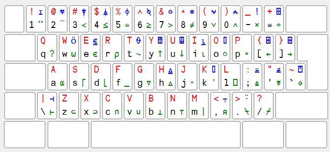
But indeed, APL code consists almost entirely of strange-looking hieroglyphics, making APL code extremely terse. This is one of the main selling points of the language - function implementations in APL are often so short that assigning a name to them seems pointless, as the name itself would be more characters than the function body.
Without further ado, let’s look at some code. I thought it would be fun as a first example to implement the function shown in the Futhark section, which calculates the length of a vector represented as an array. Here is the result:
{(+/⍵*2)*÷2}
Wow… That is pretty short. 12 characters vs Futhark’s 123, to be exact. Despite the length, quite a bit is going on here. Let’s deconstruct it.
In APL, every function takes either 1 or 2 arguments. We call these functions monadic and dyadic respectively (not to be confused with monads from languages like Haskell, which are something different). Because of this, there is no need to name function arguments - they are already named for you. ⍺ is the left function argument, and ⍵ is the right. To define an anonymous function, we use { squiggly brackets } around the function body. Looking at the snippet above, you should now see that we are defining a single argument function, which takes an argument from the right - an array, to be exact.
The first operation we perform on the input array is ⍵*2. * is the power operator, so this code will evaluate to a new array with all elements in ⍵ squared. Next, we use the squared array as the right-hand argument to the reduction operator, /. This operator takes as the left argument a binary operator, and as the right argument an array, and calculates the result of placing the binary operator between each pair of elements in the array. Concretely, +/my_array calculates the sum of elements in an array by interspersing the addition operator +. So, (+/⍵*2) calculates the sum of squares in ⍵. Lastly, we again use the power operator to calculate the square root of this sum, by using ÷2 as the exponent, which is the reciprocal of 2, ie. 0.5.
Phew, that was a mouthful. Let’s try it out in an APL REPL:
    {(+/⍵*2)*÷2}1 2 3
3.741657387
That is indeed the length of the vector [1, 2, 3]. APL array literals are simply space-separated values. To shorten this program further, we could have omitted the anonymous function and placed the argument directly into the body, like so:
(+/1 2 3*2)*÷2
We could also name our function for future use:
    vector_length ← {(+/⍵*2)*÷2}
    vector_length 1 2 3
3.741657387
An interesting property of APL, is that most operators can be used both monadically or dyadically. Take for example the iota operator, ⍳, sometimes known as the index generator. If we apply it monadically to a number n, it gives us an array of the n first numbers:
    ⍳5
1 2 3 4 5
However, when applied dyadically, it gives us the index of the right argument in the left argument. For example, we can use it to find where a number is in an array of numbers:
    8 1 4 3 2⍳3
4
Indeed, 3 is at the 4’th index of the left array.
Another interesting tidbit is that operators (and functions in general) generalize to arrays of arbitrary dimensions. This is known as rank polymorphism. In fact, we’ve already seen this in the first example program, where we used * to exponentiate an entire array. Let’s show a few more examples of this using perhaps the simplest operator of all, addition:
      1 + 5
6

      1 2 3 4 + 5
6 7 8 9

      1 2 3 + 4 5 6
5 7 9

      (1 2 3) (4 5 6) + 1 2
┌─────┬─────┐
│2 3 4│6 7 8│
└─────┴─────┘
Note the use of a 2-dimensional array in the bottom line. Fancy. In APL, anything can be thought of as an array. Even scalar numbers are just 1-element arrays. This property allows the programmer to easily apply the expressive set of operations provided by the language to any kind of data.
The building blocks described so far constitute the core of the language. Quite simple, really. Most of the features I haven’t described are pretty much just syntax sugar. The hard part of learning APL isn’t learning the language semantics, it’s learning all built-in operators and how to effectively chain them together to solve problems. Once you get the hang of it, though, APL can be a very rewarding language to write, as the time it takes to go from an idea for an algorithm to a concrete implementation can be made very short. Due to the terseness of the language, APL also excels in a REPL environment, as a sort of quick calculator on steroids.
As a final piece of piece of shilling, let me show you John Scholes famous implementation of Conway’s Game of Life in APL:
    gen←{({⊃1 ⍵ ∨.∧ 3 4 = +/ +/ 1 0 ¯1 ∘.⊖ 1 0 ¯1 ⌽¨ ⊂⍵}⍣⍵)⍺}
    R∘gen¨ ⍳4
┌─────────────┬─────────────┬─────────────┬─────────────┐
│0 0 0 0 0 0 0│0 0 0 1 0 0 0│0 0 1 1 0 0 0│0 1 0 0 0 0 0│
│0 0 1 1 1 0 0│0 0 1 1 0 0 0│0 0 1 1 1 0 0│0 1 0 0 1 0 0│
│0 0 1 0 0 0 0│0 1 0 0 1 0 0│0 1 0 0 1 0 0│0 1 0 0 1 0 0│
│0 0 1 1 0 0 0│0 0 1 1 0 0 0│0 0 1 1 0 0 0│0 1 0 0 1 0 0│
│0 0 0 0 0 0 0│0 0 0 0 0 0 0│0 0 1 1 0 0 0│0 1 0 0 1 0 0│
└─────────────┴─────────────┴─────────────┴─────────────┘
This shows the first 4 iterations of a 5x7 board initialized to a random pattern. Name another language that lets you write something like this in such a terse manner. I’ll wait.
Prolog
Selling point: Logic programming
Prolog is an interesting language primarily because it is one of relatively few languages in the paradigm known as “logic programming”. It is quite literally in the name, Pro=Programming Log=Logic. In logic programming, the programmer specifies constraints that model some problem domain, and can then execute queries against these constraints to solve problems. Prolog is best explained as a step-by-step tutorial, which is what I intend to do here.
The most basic construct in Prolog is a “fact”, denoted by an identifier, a list of operands, and followed by a dot. In the below snippet, we state several facts. Alice, Jane, Emma, and Sofia are female, while Bob, John, Lucas, and Oliver are male.
female(alice).
female(jane).
female(emma).
female(sofia).
male(bob).
male(john).
male(lucas).
male(oliver).
With this program written, we can start submitting some queries. This is typically done via a REPL. For example, we can ask whether Bob and Alice are male:
?- male(bob).
true

?- male(alice).
false
We can also ask “which people are male” by using an uppercase identifier as the input, indicating an unknown variable.
?- male(X).
X = bob
X = john
X = lucas
X = oliver
The REPL will then print all values of X which make the query true. Facts can also have multiple operands:
parent(alice, john).
parent(bob, john).

parent(jane, emma).
parent(bob, emma).
parent(jane, lucas).
parent(bob, lucas).
We can read this as “Alice is a parent of John”, “Bob is a parent of John”, “Jane is a parent of Emma”, etc. Again, we can make some simple queries:
?- parent(alice, john).
true

?- parent(bob, X).
X = john
X = emma
X = lucas

?- parent(X, john).
X = alice
X = bob
So far, so good. Now for the interesting part. Prolog’s other main construct is the “rule”. Here are some examples of rules:
father(A, B) :- parent(A, B), male(A).
mother(A, B) :- parent(A, B), female(A).
These read as:
- “A is the father of B if A is the parent of B, and A is male”
- “A is the mother of B if A is the parent of B, and A is female”
Let’s make some more queries:
?- father(bob, john).
true

?- mother(bob, john).
false

?- mother(X, lucas).
X = jane
Rules can depend on other rules, for example, we can express a grandmother constraint:
grandmother(A, B) :- mother(A, C), parent(C, B).
Which reads as “A is the grandmother of B if A is the mother of C, and C is the parent of B”. Let’s see who Oliver’s grandmother is:
grandmother(X, oliver).
X = jane
This is pretty much the core of the language, although the language does have several additional features such as arithmetics and lists. What I find cool about Prolog is that you can model your domain with it, and then use it to “explore” properties of the domain.
Although it might not seem like it from what I’ve shown, general-purpose programming is possible in the language. In some cases, we can even do better than what general-purpose languages provide. As we’ve seen, there are no functions in Prolog, just relations in the form of rules and facts. Therefore, “outputs” are typically just another variable in a relation. To illustrate this, consider the builtin for appending lists:
?- append([1, 2, 3], [4, 5, 6], X).
[1, 2, 3, 4, 5, 6]
Here, X is what we would think of as output in other languages. But since this is just a relation like any other, we can also reverse it and ask “What would we have to append to [1, 2, 3] to get [1, 2, 3, 4, 5, 6]?”:
?- append([1, 2, 3], X, [1, 2, 3, 4, 5, 6]).
X = [4, 5, 6]
We can even ask which lists append together to form [1, 2, 3, 4]:
?- append(X, Y, [1, 2, 3, 4]).
X = [],
Y = [1, 2, 3, 4]

X = [1],
Y = [2, 3, 4]

X = [1, 2],
Y = [3, 4]

X = [1, 2, 3],
Y = [4]

X = [1, 2, 3, 4],
Y = []
How cool is that? The relation works in any direction.
Here’s another example, let’s write some code that can calculate the sum of an array of integers:
sum([], 0).
sum([Head|Tail], Sum) :- sum(Tail, Rest), Sum is Head + Rest.
Readers familiar with functional programming will quickly realize this utilizes recursion. The first line states the fact that the sum of an empty list is 0. The second line is a rule consisting of 2 parts. It states that Sum is the sum of a list consisting of a Head and Tail if Rest is the sum of the Tail, and Head + Rest is equal to Sum. This way of summing a list is nearly identical to how one might do it in a LISP.
We can query it as such:
?- sum([1, 2, 3], X).
X = 6
Unfortunately, unlike the append relation, our sum is not reversible with our current implementation. This is essentially due to limitations of the is operator. There are ways to work around this using more advanced features, namely constraint solvers, but that is out of scope for this post. If this oddball programming paradigm intrigues you, give Prolog a try.